Tips for Code Organization

When analyzing electrophysiology data, you will often end up with an .Rmd file that is very long and unwieldy to scroll through. This article will provide you with some tips for good Markdown writing habits that will make your documents more manageable. I will also show you how you can use source() to refer to external .R scripts. This will make your documents even shorter and enable you to split up into different files for analyzing data, creating plots, and later, even writing different chapters of a thesis. You can even export your plots and into an attractive, easy-to-read HTML document to make it easy to show to others.

Tip 1: Use Markdown headers

Markdown is a plaintext writing language that you are probably already familiar with from writing online. You can use two **asterisks** to make text bold, or one set each for italicized text. You can use hashtag symbols (#) to specify headers.

For example, let’s say that your coding document has the following structure:

• Data analysis
  • Evoked current data
    • Amplitudes
    • PPR
    • Variance data
  • Spontaneous current data
  • Action potentials
• Plots

Try it out! Create an empty .Rmd file and write down the following sample outline:

# Data analysis

## Evoked current data

### Amplitudes

### PPR

### Variance

## Spontaneous current data

## Action potentials

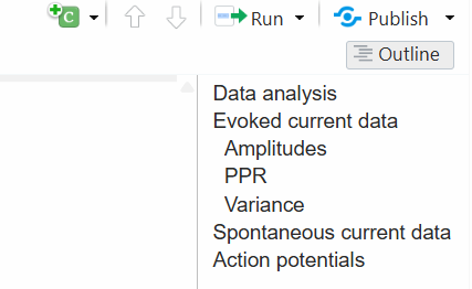
The headings should change to a different colour in RStudio. You can now use the Outline tool, available as a pop-up in the upper-right corner of the screen.

Tip 2: Name your chunks

You can name code chunks which will assist with navigation and make error tracing easier.

So instead of this:

```{r}

```

Type this:

```{r import-data}

```

After the chunk name, you can also type a comma and then use chunk options like fig.width=7, fig.height=5, eval=FALSE, etc.

```{r import-data, message=FALSE}

```

The author of the knitr package has listed all the chunk options and how to use them on their knitr chunk options page.

Note! Ensure that you do not duplicate any chunk names, or R will display warnings when trying to knit the document.

Note! The chunk names must not have any spaces or start with a number.

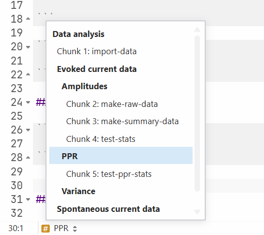
Now you can use the navigation bar at the bottom left of the Source pane to quickly jump to different code chunks or use Ctrl+F to search for the chunk!

Tip 3: Learn keyboard shortcuts!

You probably already know shortcuts like Ctrl+C to copy and Ctrl+V to paste, but there are some shortcuts specific to RStudio that will speed up your coding time.

Inserting a chunk

For example, use Ctrl+Alt+I (or Cmd+Alt+I on a Mac) to quickly insert a new empty R chunk.

```{r}

```

Inserting a pipe symbol

To insert the pipe symbol %>% when stringing functions together, use Ctrl+Shift+M. It is faster than reaching for the % key!

Inserting the assign symbol

Use the assign symbol (less-than sign then a hyphen <-) not the equal sign (=) when naming variables. For example, use x <- 2 not x = 2. You can use the Alt+- (alt + hyphen key) to quickly insert this symbol.

Run code in a chunk only

You do not have to highlight/select a line of code to run it! To run the code in one chunk only, place your cursor anywhere in the chunk and type Ctrl+Shift+Enter. To run only a single line, put your cursor at the end of it and type Ctrl+Enter.

You can also put your cursor at the end of a dplyr series of functions (frequently connected by the %>% symbol) or ggplot code and press Ctrl+Enter to run the function or generate the plot.

Switch between panes

It can be handy to switch between the Source pane (where you are writing code and text) to the Console pane (handy for quick calculations, math, and testing code that you don’t want to keep). Use Ctrl+1 and Ctrl+2 to jump from one pane to the other. It will automatically jump your cursor into the available space and you can start typing!

Comment/uncomment lines

Select code that you don’t want to run and then use Ctrl+Shift+C to comment out all the lines in one move.

Jump to any file or function

Use Ctrl+. to open a search box. As you type, it will bring up functions, code snippets, and files within your R project!

Clean up code

Use Ctrl+Shift+A to automatically clean up messy or cramped code and adjust the spacing according to good coding practice. This brings me to the next tip!

Tip 4: Clean up your code

Good coding practices include things like including spaces before and after operator signs. For example, write x <- 2 + 2 not x<-2+2.

If you are using ggplot2 you should end each line with the + symbol then start the next line. Each layer (whether it is data, labels, or formatting) should have its own line.

This is an example of properly formatted code.

penguins %>%
  ggplot(aes(x = bill_len, y = flipper_len, colour = species)) +
  geom_point(size = 3, alpha = 0.7) +
  labs(x = "Bill length (mm)", y = "Flipper length (mm)", colour = "Species") +
  theme_minimal() +
  theme(
    axis.title.x = element_text(size = 15, margin = margin(t = 20)),
    axis.title.y = element_text(size = 15, margin = margin(r = 20))
  )

It is good to get into these habits as you are writing code, but there are also handy tools to format code after it is written.

RStudio has a built in code formatting tool. Use Ctrl+Shift+A to clean up selected code or use Code -> Reformat selection.

Tip 5: Use an R project and keep it organized

If you have set up your document using the instructions on the Getting Started page, you should hopefully already have an RProject set up. I encourage you to keep it maintained.

• Open RStudio every time using your .Rproj file, or once you have RStudio open, click on File -> Open Project. This will allow you to use the here package to easily refer to files in subfolders with relative paths (e.g. Data/Raw-CSVs/20240503-Raw-Data.csv) instead of absolute paths (e.g. C:/Users/cslau/OneDrive/Desktop/Masters-Work/masters-thesis/Data/Raw-CSVs/eEPSC-Data/20240503-Raw-Data.csv).

• Keep folders specific (e.g. Data, Figures, Paper) and only put things in them that belong there.

• Keep your README.txt file up to date so that when you look at it years later, you can quickly orient yourself to what is in each folder and what the project is about. The README file should be a simple, plaintext document with a description about the project, names and contact info, and a brief summary of the folders and their contents.

Tip 6: Prevent clutter in R and your code

It is important that you do not have old variables, loaded packages, and other named objects cluttering your environment. The code should only include the packages and variables that you need for this project.

In Tools -> Global Options be sure to UNCHECK Restore .RData into workspace at startup and set Save .RData to workspace on exit to NEVER. R will shut down and open faster.

To speed up loading time when you open RStudio, you can also uncheck Restore most previously opened project at startup and Restore previously open source documents at startup, but this does mean you will have to open them each time. I recommend this only if you find that RStudio is slow to open, or if you like having a clean slate each time.

To prevent old variables and named objects from cluttering your environment, frequently click on the drop-down arrow next to the Run button and click on Restart R and Clear Output.

As you are coding, you will develop new ways to make your code as streamlined as possible. It is sometimes fun to see how short you can make your code. For example:

• Could you use functions like across() from dplyr instead of repeating the same function for each column?
• Do you need to use all the arguments for a function, or are the default values (visible in the help page for the function) sufficient?
• If you have to repeat code multiple times, you should write a custom function or find ways to shorten it. If you come from other coding languages, you may want to use loops, but R is even more efficient with lists. Consider storing items in lists and then running a function on each element of that list. For example c(1, 2, 3) + 2 will automatically add 2 to each element of the list, resulting in c(3, 4, 5).

Tip 7: Set common settings once

Instead of repeatedly writing chunk settings like echo=FALSE for each chunk in your document, set this in a chunk at the top of your document and it will apply to all chunks below. Here is an example of what my setup chunk often looks like:

knitr::opts_chunk$set(
  dev = "png",
  fig.align = "center",
  out.extra = "",
  out.width = "75%",
  dpi = 300,
  comment = NA,
  message = FALSE,
  warning = FALSE,
  echo = FALSE
)

The comment = NA will remove the double # symbols that R prints out when displaying results. Set FALSE for message, warning, and echo. This will print the output of the chunk (numbers, plots, etc.) but hide the chunk itself and any messages/warnings. You’ll still see them when running them yourself in R. Feel free to change the dpi (dots-per-inch) if needed.

The setup chunk can get very long and specific. Here is an example of the setup chunk for my thesis, where I had some settings specific to making a nice PDF. The fig.path option enables output figures to go to a subfolder.

knitr::opts_chunk$set(
  dev = c("cairo_pdf"),
  dpi = 600,
  fig.width = 12,
  fig.height = 12,
  out.width = "\\linewidth",
  fig.align = "center",
  comment = NA,
  message = FALSE,
  warning = FALSE,
  echo = FALSE,
  fig.path = "Thesis-Figures/"
)

Tip 8: Source your documents

Right after your setup chunk, I strongly suggest having separate .R scripts for data import, statistical analysis, and plot generation. This will make them shorter and you can just source these scripts anywhere you want to have the data available. You could even consider having an .R script called Libraries.R to load commonly used libraries and reduce repetition.

Create an .R file and copy the content of the chunks (only the content, not the chunk labels or settings, or closing backticks). Consider creating R scripts like Import-data.R and Make-plots.R.

Now, how do you get the data into your R environment in a separate document? You must source these script files in the correct order. For example, Make-plots.R will give you errors if you try to run it before you’ve sourced Import-data.R.

At the top of your thesis document, create a chunk where you source these scripts. I have kept my .R files in the Scripts subfolder of my project so that is why I have Scripts/ in the filepath. It will look like this:

source(here::here("Scripts/Import-Data.R"), local = knitr::knit_global())
source(here::here("Scripts/Plot-generator.R"), local = knitr::knit_global())

It is important to have the local = knitr::knit_global() statement because this will enable R to include these scripts (and the data and plots they produce) while knitting your document to a PDF or HTML.

Tip 9: Use the patchwork package or facet plots

You can use the patchwork package to put multiple plots together. Install the package and then load it with library(patchwork). You can then present multiple plots in one chunk by adding them together.

For example p1 + p2 will result in two plots displayed side-by-side, and (p1 + p2)/(p3 + p4) will result in a grid of four plots arranged in a 2 pattern. I encourage you to read the patchwork package website for more useful tips!

Here is an example. I used fig.width = 12, fig.height = 10 in the chunk options.

(raw_plot + summary_plot)/
  (ppr_plot + ap_trace)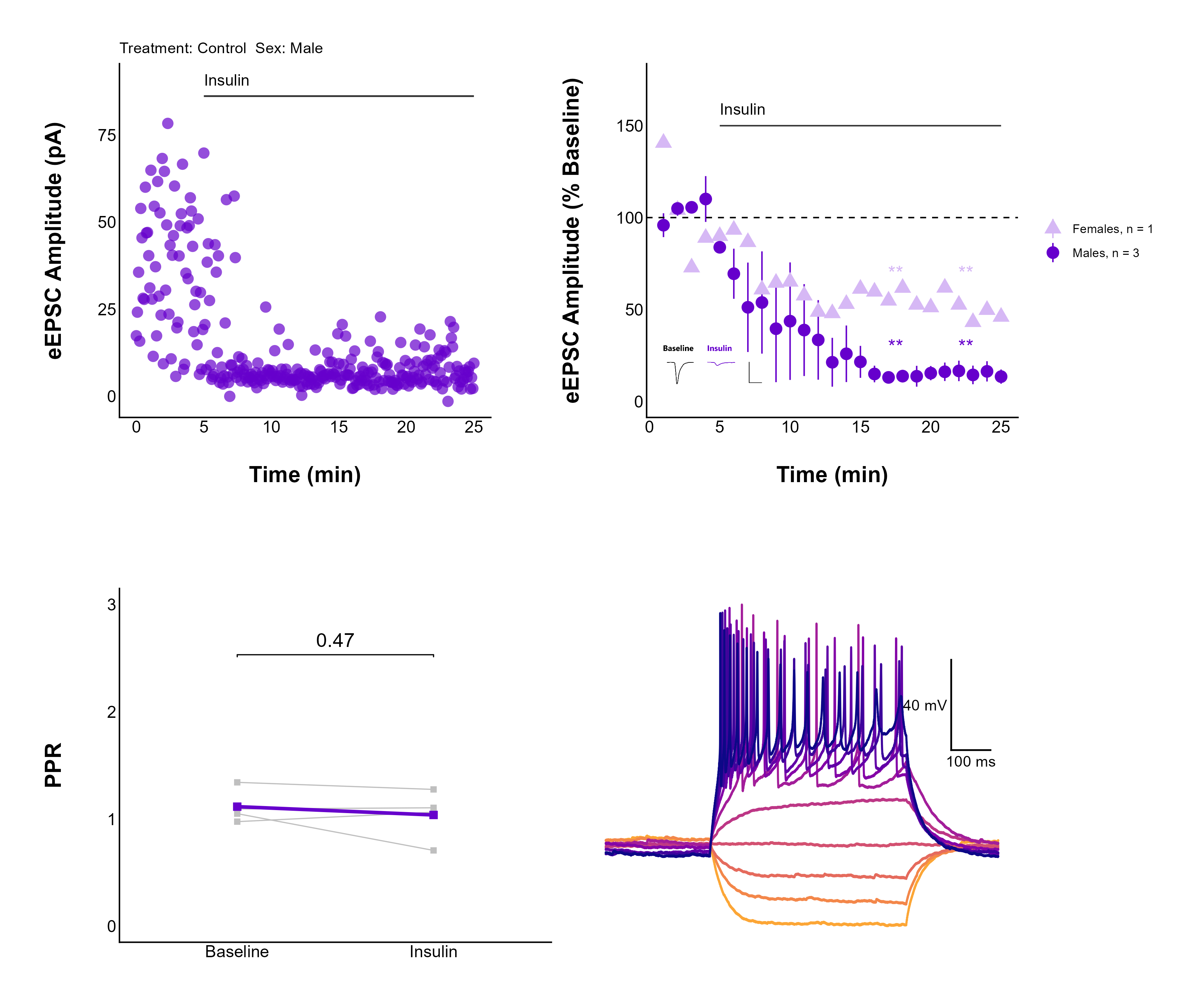

To add figure captions, just add the plot_annotation() function. Previously I also defined a ggplot theme that makes the figure captions bold:

patchwork_theme <- theme(plot.tag = element_text(
  size = 18,
  margin = margin(r = 8, b = 8),
  face = "bold"
))

Use the + sign to add the plot_annotation and use the & symbol to add a ggplot theme (your own or a pre-built theme).

patchwork_example_2 <- (raw_plot + summary_plot)/
  (ppr_plot + ap_trace) + plot_annotation(tag_levels = "A") & patchwork_theme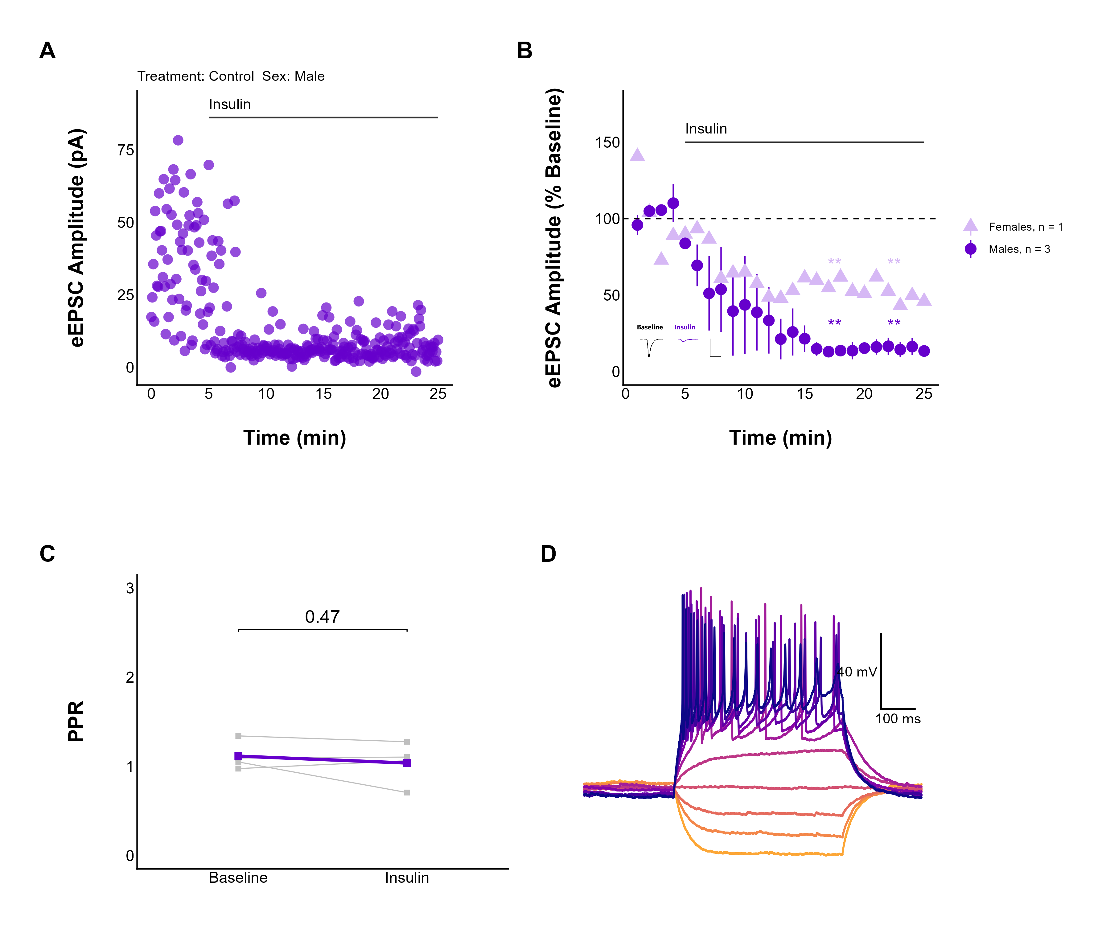

To add a figure caption, use the fig.cap = "Insert figure caption here" chunk option.

Pro tip! If your figure caption gets too long, you can separate out knitr chunk options onto separate lines using #|. I will show an example below:

#| insulin-plots,
#| fig.cap = "Sample insulin plots A) Raw evoked current plot
#| B) Summary evoked current plot
#| C) PPR plot
#| D) Action potentials plot.",
#| out.width = "100%"

(raw_plot + summary_plot)/
  (ppr_plot + ap_trace) + plot_annotation(tag_levels = "A") & patchwork_theme

If your figure captions get too long, I highly recommend naming them as separate objects with names like chapter_2_fig_1_cap so you can easily refer to them.

chapter_2_fig_1_cap <- "Sample insulin plots A) Raw evoked current plot, B) Summary evoked current plot, C) PPR plot, D) Action potentials plot."

Tip 10: Showcase your work!

This last tip is the culmination of all former tips. It will help you display your data in an attractive, convenient way – using HTML!

When you want to show your data and plots to others, it can be awkward to scroll through long script files and re-run chunks to show plots. I highly recommend creating a simple document focused only on presenting the key facts. This could include:

• A table of cell counts per group and sex
• A series of plots of your raw data with separate tabs for each sex (use .tabset next to the header to make all subheadings appear on separate tabs!).
• Summary plots per group and sex

The last two would be repeated for as many groups that you have, separated by headers. Ideally this document would have a table of contents so you can jump quickly to the group you want to examine.

The document will have the following chunks:

• The setup chunk
• The chunk where you source external scripts for importing your data and making plots
• A chunk for displaying the table of your cell counts (hint: use the summary data $mean_SE from make_summary_current_data!)
• A chunk displaying the raw plots
• A chunk displaying the summary plots

The last two chunks would be repeated for as many groups that you have, separated by headers. Ideally this document would have a table of contents so you can jump quickly to the group you want to examine.

To make this document, click the Knit button and choose HTML (the next time you do this, it will automatically choose HTML for you). You can customize this with your own .css file or choose from the many themes available by default. I’ve included an example of how you could change the html theme and enable a floating table of contents.

---
title: "Plot Viewer"
author: "Type your name here"
date: "September 08, 2026"
output: 
  html_document:
    theme: cosmo
    toc: true
    toc_depth: 3
    toc_float:
      collapsed: false
      smooth_scroll: false
---

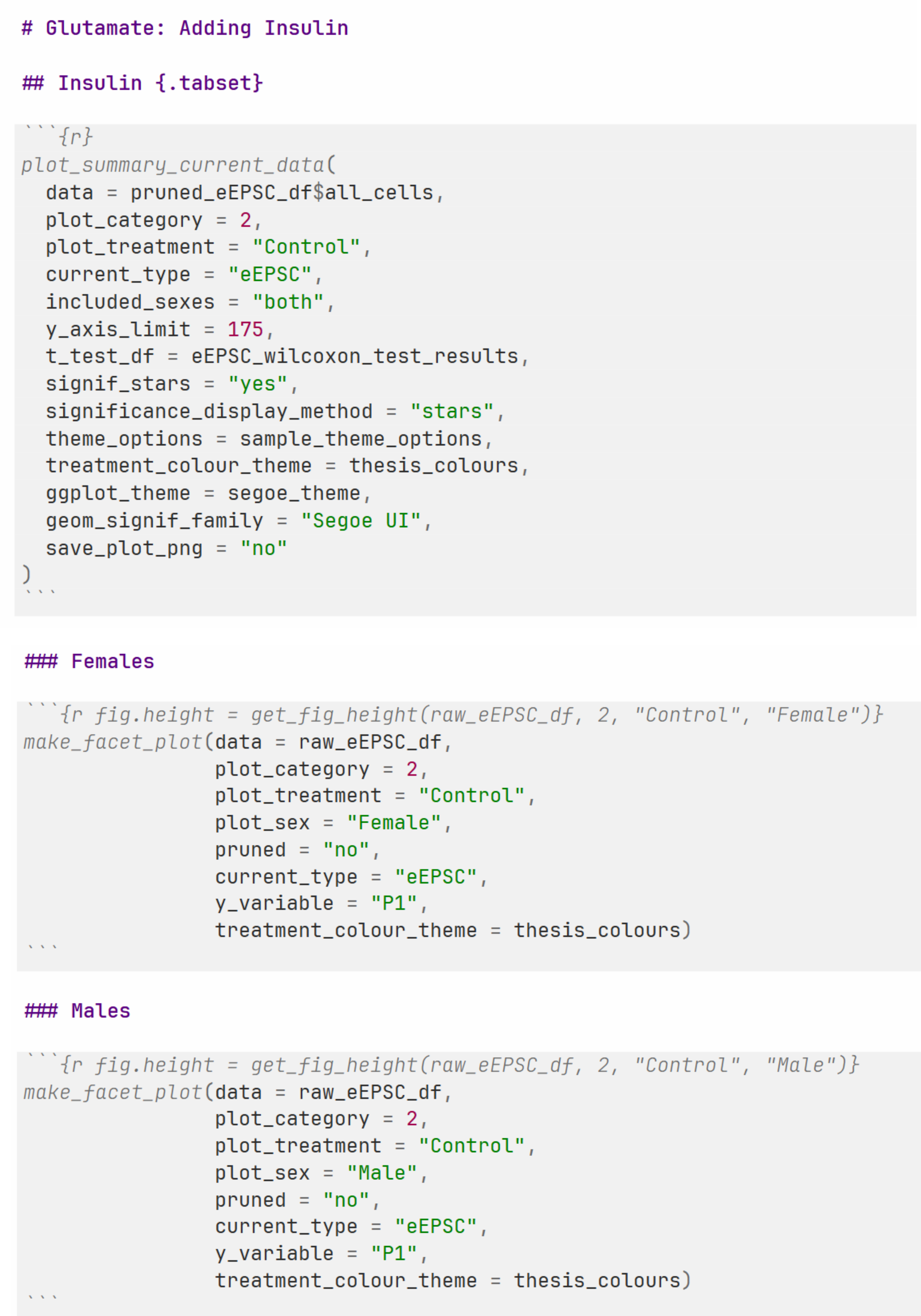
To help get you started, I’ve included an excerpt of what part of this document could look like from my own Plot-Viewer.Rmd file: