
Action Potential Analysis
Source:vignettes/articles/action-potential-analysis.Rmd
action-potential-analysis.RmdThis vignette will demonstrate how to analyze action potential
properties in Clampfit using a raw .abf file. You will identify the
first current injection that resulted in action potentials and then
select the first action potential within this sweep for further
analyses. The data can then be processed and plotted in R using
patchclampplotteR functions.
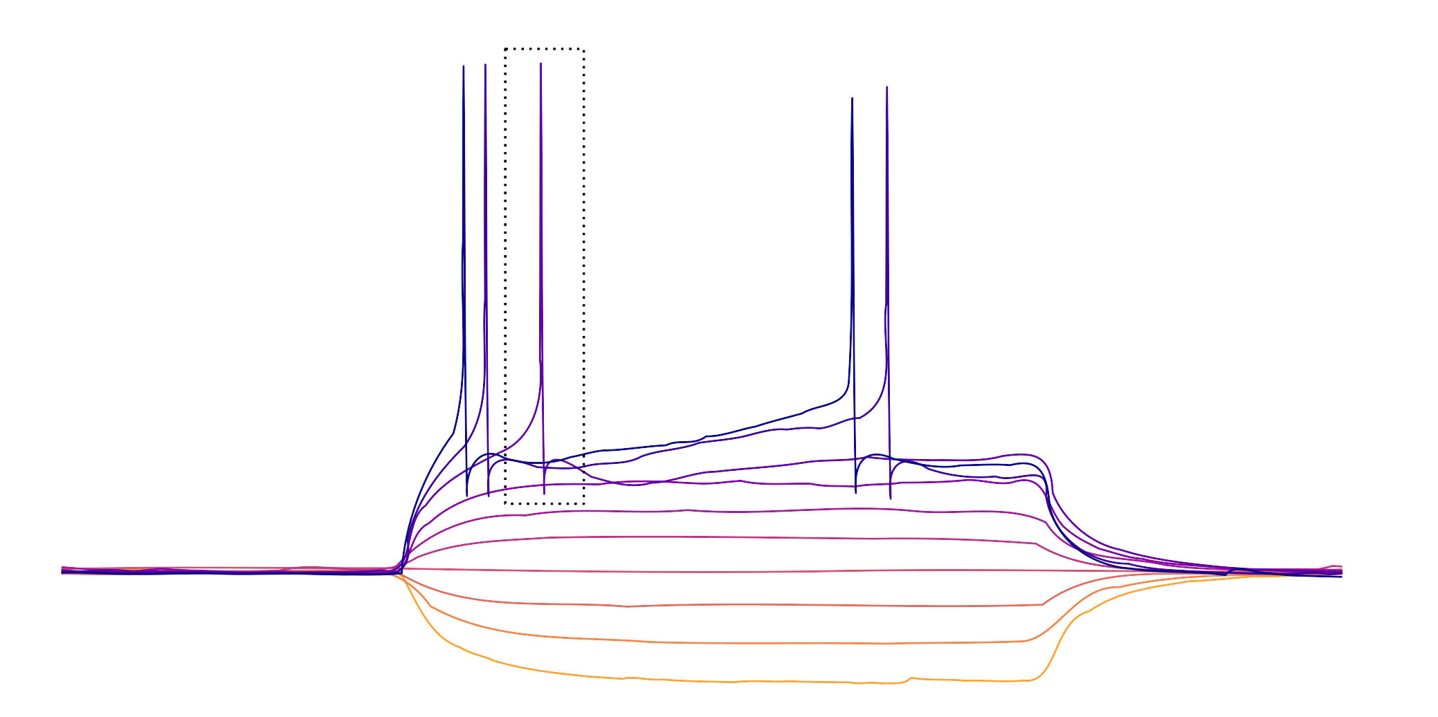
The box outlines the first action potential on the first sweep with action potentials.
You will identify the threshold using the first derivative method. This means that the threshold corresponds to the membrane potential where the action potential velocity is 10 mV/ms or greater (Farries et al., 2010).
Set up data sheet
Before you begin, you should set up a .csv file. I would suggest
using a consistent naming scheme that includes the date. I use the
YYYYMMDD-title.csv format, such as
20250113-AP-analysis.csv. This makes it easy to identify
when I last analyzed my data, and the files sort easily.
In your .csv file, fill row 1 with the following column titles.
Notice that all (except for ID are in lowercase.
-
letterThe unique letter identifier of a single cell. You can use this to link data from different recordings taken from the same cell. -
stateA character value. In this example, the values areBaselineandInsulin, indicating a current clamp protocol taken after the cell had been exposed to 500 nM insulin for 25 minutes. -
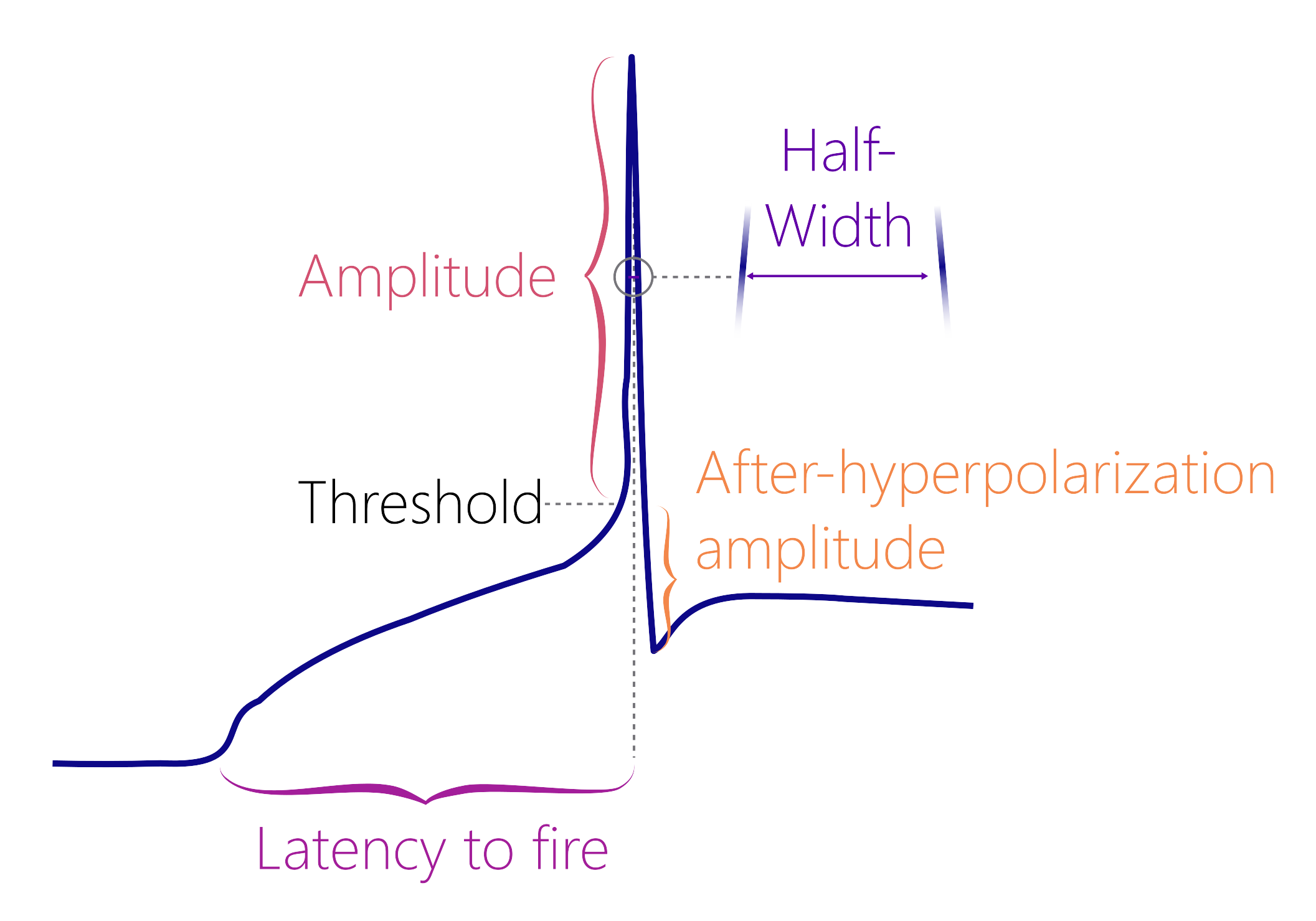
time_of_thresholdA numerical value (in ms) used to determine properties like the latency to fire. -
t_xThe membrane potential at the moment that an action potential is initiated, also known as the threshold. -
t11The derivative of the trace you are analyzing. Must be 10 mV/ms or greater to properly identify the threshold. -
IDA character value indicating the recording number. This corresponds to theFile Namecolumn that is automatically generated in the Results sheet in Clampfit. -
first_sweep_with_APsA number representing the earliest sweep number where action potentials first appeared. -
trace_startThis is an automatic value calculated by Clampfit, and it corresponds to the sweep number. It is not used in any analyses, but it will automatically be included in the Results sheet in Clampfit. It’s faster to just copy all the data rather than try to exclude this value. -
peak_amplitudeThe membrane potential (in mV) during maximum depolarization. -
time_to_peakThe time of the peak amplitude (in ms), which should also be relative to thetime_of_thresholdif you have repositioned Cursor 1 to thetime_of_threshold. -
antipeak_amplitudeThe afterhyperpolarization amplitude (in mV) -
time_of_antipeakThe time of the after-hyperpolarization (in ms), which should be relative to thetime_of_threshold. -
half_widthThe width of the action potential when the membrane potential is half of thepeak_amplitude. -
ap_notesAn optional column where you can note any unusual or interesting things about the recording, or flag a nice-looking recording for use in a paper.
Get derivative
- Open the .abf file containing the current clamp step protocol in
Clampfit. Ensure that the x-axis shows time in milliseconds. If it shows
seconds, double-click the x-axis, and change the
Elapsed TimefromAutomatictoMilliseconds.
Warning! The y-axis values should generally be around -70 mV during the flat regions outside of the current injection. Sometimes the scaling factor in Clampfit is distorted (for unknown reasons) and the y-axis may be in the thousands range. If this happens, follow step 1b).
1b. If the y-axis scale is off (see the warning box above),
double-click on the y-axis to open the
Modify Signal Parameters box. Change the V/pA
ratio to 0.01, and click “Save” and then “OK” (you will see a warning
about permanently changing the recording - don’t worry about this, and
just be sure to say “no” to saving changes when closing the file later).
This will re-scale the y-axis to the correct units relative to the
current injections. Double-check that the x-axis is in milliseconds!
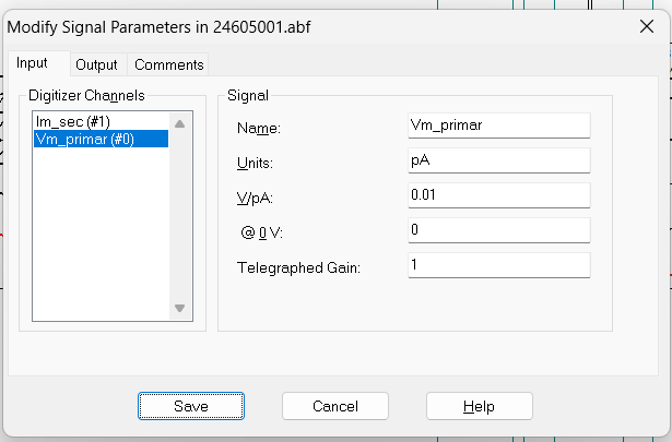
Sometimes the V/pA ratio is altered, so you may need to change it to 0.01.
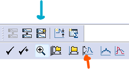
1c. Click on the Show Aquistion Signals button and then
Previous Signal (blue arrow in the figure below) to view
the sweeps showing changes in current (Vm_primary). The
traces should all be stacked on top of each other, but if they are not,
click on View -> Data Display ->
Sweeps.
1d. You can also click on the Auto Scale All Y Axes
button (orange arrow) to help you see the data faster.
Press the “Enter” key to show just one sweep at a time. It will begin at the sweep corresponding to the lowest current injection. Use greater than symbol (
>) to cycle up through the sweeps.Move up to sweeps corresponding to higher current injections until you identify the first sweep that contains an action potential. I will call this
t_x, since it may bet5in one recording, ort6in another, etc.Position Cursors 1 and 2 around the first action potential in
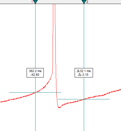
t_x. Cursor 1 should be before the threshold (aim for the area before the slope of the curve increases steeply). Cursor 2 should be in the after-hyperpolarization region.
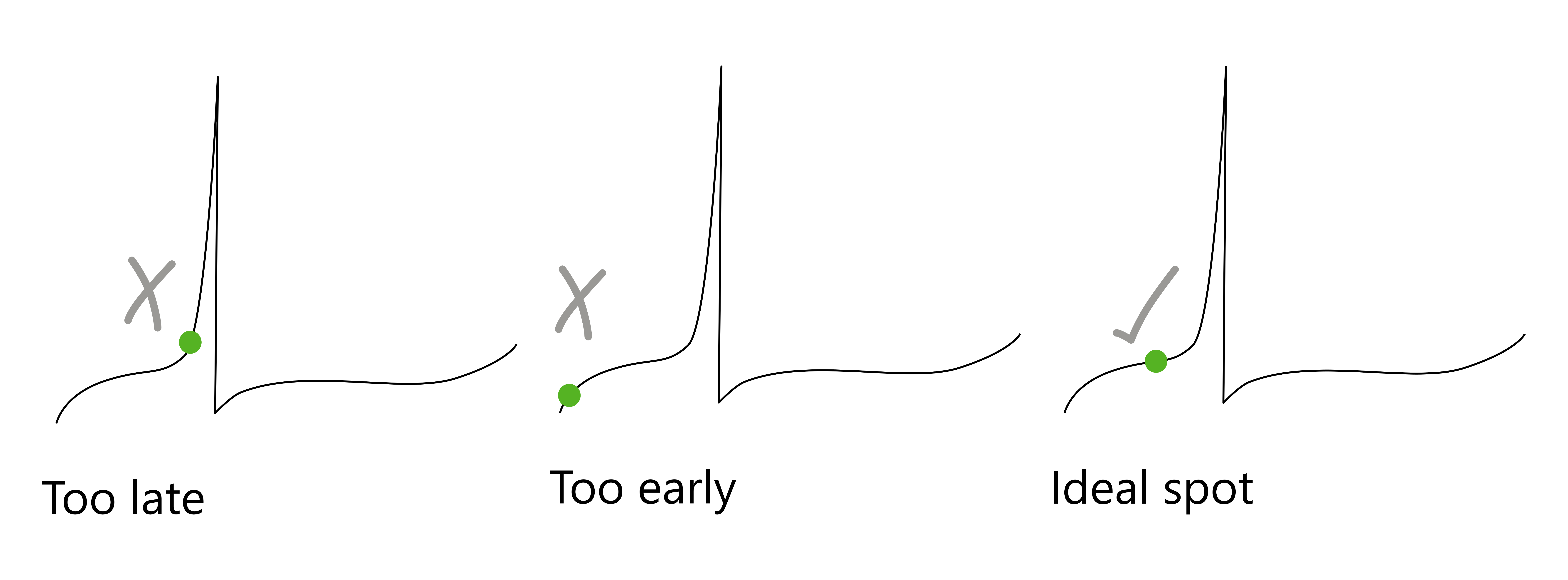
The ideal placement of Cursor 1 should be in the middle of the curve. Left: Cursor 1 is placed where the curve is very steep, and it is likely that you will miss the threshold. Middle: Cursor 1 is very low, so Clampfit may identify this as the after-hyperpolarization. Right: This is the ideal spot, where the cursor is early enough to capture the threshold in the search region.
Warning! It is important that Cursor 2 touches the curve at a value that is lower than the voltage value for Cursor 1. If Cursor 1 is lower, then Clampfit may identify the location at Cursor 1 as the after-hyperpolarization region if you forget to move the cursor to the threshold (see step 11).
Also, make sure that Cursor 2 does not cross a second action potential. The range between Cursors 1 and 2 should only cover one action potential.
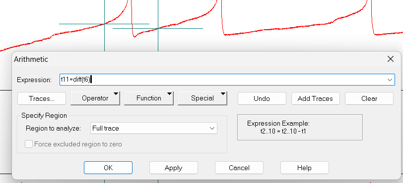
Click on the arithmetic button (it is the button with basic math symbols), then Add Traces. Write “1” and click OK. This will add a new empty trace, called
t11.t11should be the derivative oft_x. In theExpressionbox, writet11=diff(t6)(replacet6with your value fort_x).
Find threshold
- Click on
Edit->Transfer Tracesand set theRegion to transferasCursors 1..2. In theTrace Selectioncategory, choose onlyVm_primary ()as the signal. Ensure thatstart time at zerois checked. Selectt_xandt11for the traces, then clickOK.
Quick Tip! An even faster keyboard shortcut is
Alt+e+t+s, which will immediately open the correct signal selection box. Only use this if you are sure that the settings are correct.
- Click on the Results sheet (
Window->Results1orAlt+w+2). TheResultspage will display three columns:Time (ms),Trace #6 (or #5, #7, etc.), andTrace #11.Trace #xis the membrane potential in mV, andTrace #11is the derivative ofTrace #x.
Warning! The Results page of the transferred traces does not delete data between files. If you are doing several analyses in one session, ensure that you are looking at the correct columns corresponding to the active recording.
Note If you recently opened a results file in Clampfit, it will automatically overwrite the contents of Sheet 14, and you will not see the transferred traces. If you don’t see any results, you may need to close and re-open Clampfit.
- Scroll down the
Trace #11column (the derivative column) until you see a series of positive values with increasing magnitude (e.g. > 100 or more). This is where the derivative is increasing. Select the first value within this series that is greater than or equal to 10 mV/ms. Copy the value of all three columns in this row.
Note There may be isolated peaks within the derivative that are greater than 10 mV/ms. Only select this value if it is part of a series of increasingly larger positive values, followed by a series of negative values.
- If the scaling is correct, the threshold (
t_x) should be around -30 mV for a healthy cell. Your .csv file should now look like this:
Measure action potential properties
- Double-click on Cursor 1 and change its x-position value
(
time) to match thetime_of_threshold.
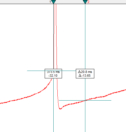
Note how Cursor 1 is shifted to the right relative to the earlier cursor image. It is now located at the x-value where the membrane potential crosses the threshold.
Warning! If you do not reposition Cursor 1 to be at the time of threshold, the values for
time_of_peakandtime_of_antipeakwill be incorrect!
You don’t need to move Cursor 2 if it is correctly positioned from earlier steps (it should be in the after hyperpolarization region, lower than Cursor 1, and not touching a second action potential).
Click on the Statistics button (a small icon with a summation symbol on top of it) or press
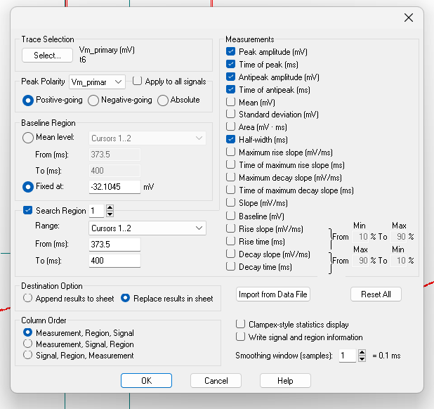
Alt+s.Set the following settings:
- Trace Selection: Choose
Vm_primary ().t_xandt11will automatically be selected. - Peak Polarity:
Vm_primary,Positive-going - Baseline Region: Fixed at
[paste in the threshold value (column t_x in your sheet) here] - Search Region 1: Range:
Cursors 1..2 - Destination Option:
Replace results in sheet(prevents you from accidentally copying old data - Column Order:
Measurement, Region, Signal - Measurements:
peak_amplitude,time of peak,antipeak amplitude,time of antipeak,half-width
Click OK and then Window -> Results1
(Alt+w+2) to see the Results page.
- Go to the row corresponding to Trace
t_x. Select all data except for theFile Pathcolumn (unless you think you will need it later) and paste it into the .csv file. You’ll notice that the .csv column names are different than the column names in theResultssheet. I changed these column names to make them easier to use in R code.
Warning! There is a bug in Clampfit 11.3 (but not 11.4 or 10.6) that leads to incorrect time units for parameters such as time_of_antipeak. Ensure that your parameters have consistent units before moving ahead!
- Your .csv file should now look like this.
While you still have this file open, you may want to count action potentials (see the section on counting action potentials below). Or, you could wait and do these separately, which you might find more efficient.
A completed dataset should look something like the spreadsheet below.
Note If there are no action potentials in the later recording, insert the values for the columns
letterandstateand leave all the others blank.
You are now ready to import your data into R! Use the
add_new_cells()function withdata_type = "AP_parameter". You may find it helpful to read the Get Started guide if you are setting up your data for the first time.Use the
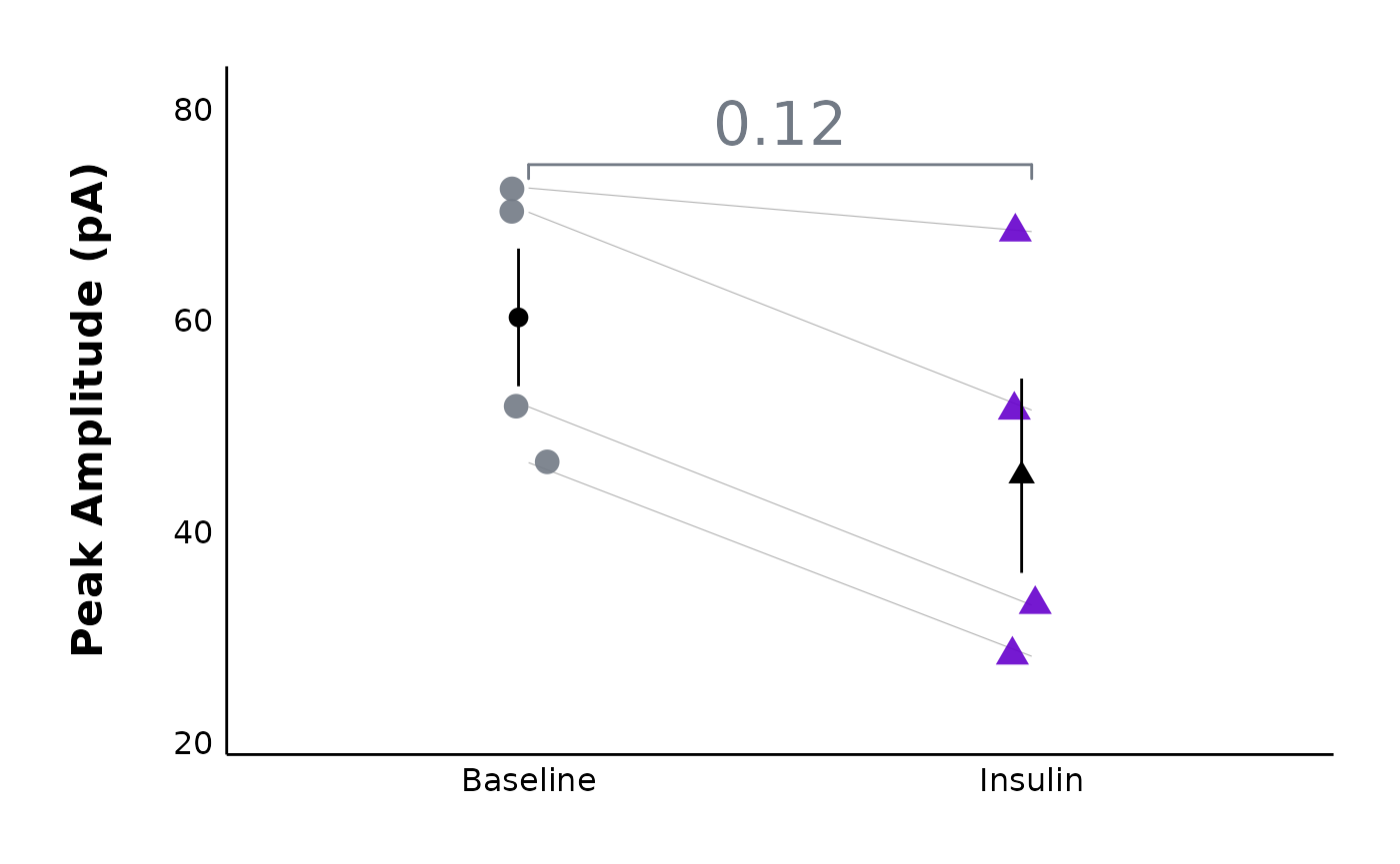
plot_AP_comparison()function to see how parameters likepeak_amplitudeandhalf-widthchange after your treatment.
plot_AP_comparison(
  sample_AP_data,
  plot_treatment = "Control",
  plot_category = 2,
  y_variable = "peak_amplitude",
  y_axis_title = "Peak Amplitude (pA)",
  theme_options = sample_theme_options,
  baseline_label = "Baseline",
  test_type = "wilcox.test",
  post_hormone_label = "Insulin",
  treatment_colour_theme = sample_treatment_names_and_colours,
  save_plot_png = "no"
)
Count action potentials
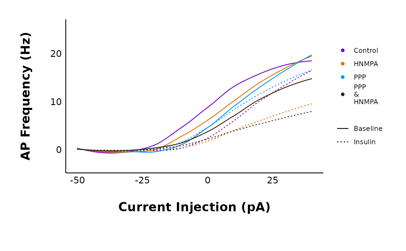
The next step is to count the number of action potentials in each sweep. This will allow you to later make a plot of action potential frequency vs. current injection and see how a treatment affect action potential frequency.
- Create a separate .csv file (for example
20250113-AP-count-data.csv). This file should have four columns:
-
letterThe unique letter identifier of a single cell. -
stateA character value (“Baseline” or “Insulin” in this example) -
sweepA number from 1 to 10 (see step 18a to generate this) -
no_of_APsa numerical value indicating the number of action potentials
18a. To generate a repeated sequence from 1-10 quickly, type the
number 1 in cell C2. Then, type the number 2 in cell
C3.
18b. Select C2 and C3 together, then hover
your mouse over the bottom right corner of the group until you see a
small black plus symbol.
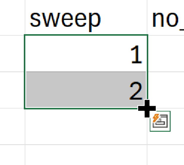
18c. Click and hold down the mouse key and drag the selection down to
C11 to generate a sequence from 1 to 10.
18d. The entire range from C2 to C11 should
be selected. Move your mouse to the bottom right corner of the cell
until you see the + symbol again. Hold down the
Ctrl key and drag this selection down. This will generate
the sequence from 1-10 repeatedly (e.g. 1, 2, 3, 4, 5, 6, 7, 8, 9, 10,
1, 2, 3…)
18e. You can then copy and paste this range repeatedly to fill your column.
- Open a current clamp steps recording in Clampfit (you may be coming directly from step 16 when you measured action potential properties).
19b. Ignore these instructions if you’ve already set up the plot
view You may need to zoom in to see it better. Click on the
Show Aquistion Signals button and then
Previous Signal (blue arrow in the figure below) to view
the sweeps showing changes in current (Im_primary ()). The
traces should all be stacked on top of each other, but if they are not,
click on View -> Data Display ->
Sweeps. You can also click on the
Auto Scale All Y Axes button (orange arrow) to help you see
the data faster.

- Press the
Enterkey to view one sweep at a time, and use<and>to cycle through the sweeps. Count the number of action potentials in each sweep, and record them in theno_of_APscolumn.
Yes, this step may seem super simple, but that’s because it is - look at each sweep and count the number of action potentials present!
20b. Tip! If there are no action potentials in a sweep,
leave the cell in your Excel sheet blank. After you have finished
collecting data from many cells, you can automatically fill blank cells
with 0.
20c. Select the no_of_APs column. Then, click on
Home -> Editing ->
Find and Select -> Go to Special and then
choose Blanks.
20d. All of the blank cells should be selected. Type the number
0, and then press Ctrl + Enter or
Cmd + Enter on a Mac. All blank values should be filled
with 0s now.
- Here is an example of what one recording could look like:
You are now ready to import the data into R! Use
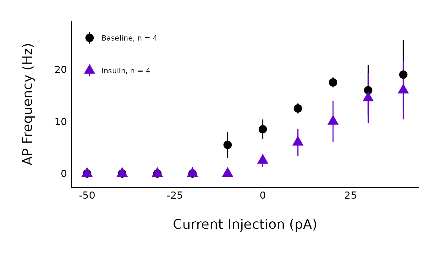
add_new_cells()withdata_type == "AP_count".Here is an example of the type of plots you can create!
plot_AP_frequencies_single_treatment(
  data = sample_AP_count_data,
  plot_treatment = "Control",
  plot_category = 2,
  baseline_label = "Baseline",
  hormone_added = "Insulin",
  significance_display_method = "stars",
  treatment_colour_theme = sample_treatment_names_and_colours,
  large_axis_text = "no",
  test_type = "wilcox.test",
  theme_options = sample_theme_options,
  save_plot_png = "no"
)
plot_AP_frequencies_multiple_treatments(
  data = sample_AP_count_data,
  include_all_treatments = "yes",
  plot_category = 2,
  treatment_colour_theme = sample_treatment_names_and_colours
)
Plotting Sweeps
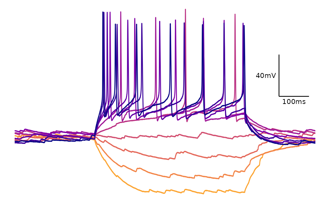
You can plot action potential recordings using
plot_AP_traces(). Use a dataframe generated using
import_ABF_file() with
recording_mode = "current_clamp". You can then plot all
sweeps using
sweeps = as.character(unique(sample_ap_abf_baseline$episode)).
Just replace sample_ap_abf_baseline with the dataframe that
you inserted into the data argument. Set
colour_scale_option to one of three options: “viridis”,
“custom” or “single_colour”.
Viridis
“viridis” enables the beautiful colourblind-friendly viridis palettes
from the viridis package. Look at the documentation
for scale_color_viridis to learn about options you can
use. These include begin, option,
theme and more.
plot_AP_trace(
  data = sample_ap_abf_baseline,
  sweeps = as.character(unique(sample_ap_abf_baseline$episode)),
  colour_scale_option = "viridis",
  plot_category = 2,
  plot_treatment = "Control",
  direction = -1,
  option = "plasma",
  begin = 0,
  end = 0.8
)
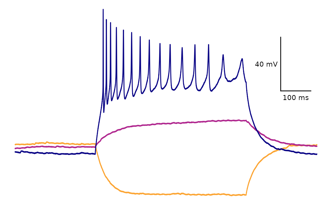
This is how you would plot selected sweeps. Include a list of one or more values corresponding to the sweep names (“epi1” to “epi10” in this example).
plot_AP_trace(
  data = sample_ap_abf_baseline,
  sweeps = c("epi1", "epi5", "epi10"),
  colour_scale_option = "viridis",
  plot_category = 2,
  plot_treatment = "Control",
  direction = -1,
  option = "plasma",
  begin = 0,
  end = 0.8
)
Custom scale
If you use colour_scale_option = "custom" you must
define a list of character values (can be hex values or named colours)
in the custom_scale_colours argument.
plot_AP_trace(
  data = sample_ap_abf_baseline,
  sweeps = as.character(unique(sample_ap_abf_baseline$episode)),
  custom_scale_colours = c("#edd03a", "#cced34", "#a3fd3d", "#6bfe64", "#31f199", "#18dcc3", "#29bbec", "#4294ff", "#466be3", "#4040a2"),
  colour_scale_option = "custom",
  plot_category = 2,
  plot_treatment = "Control"
)
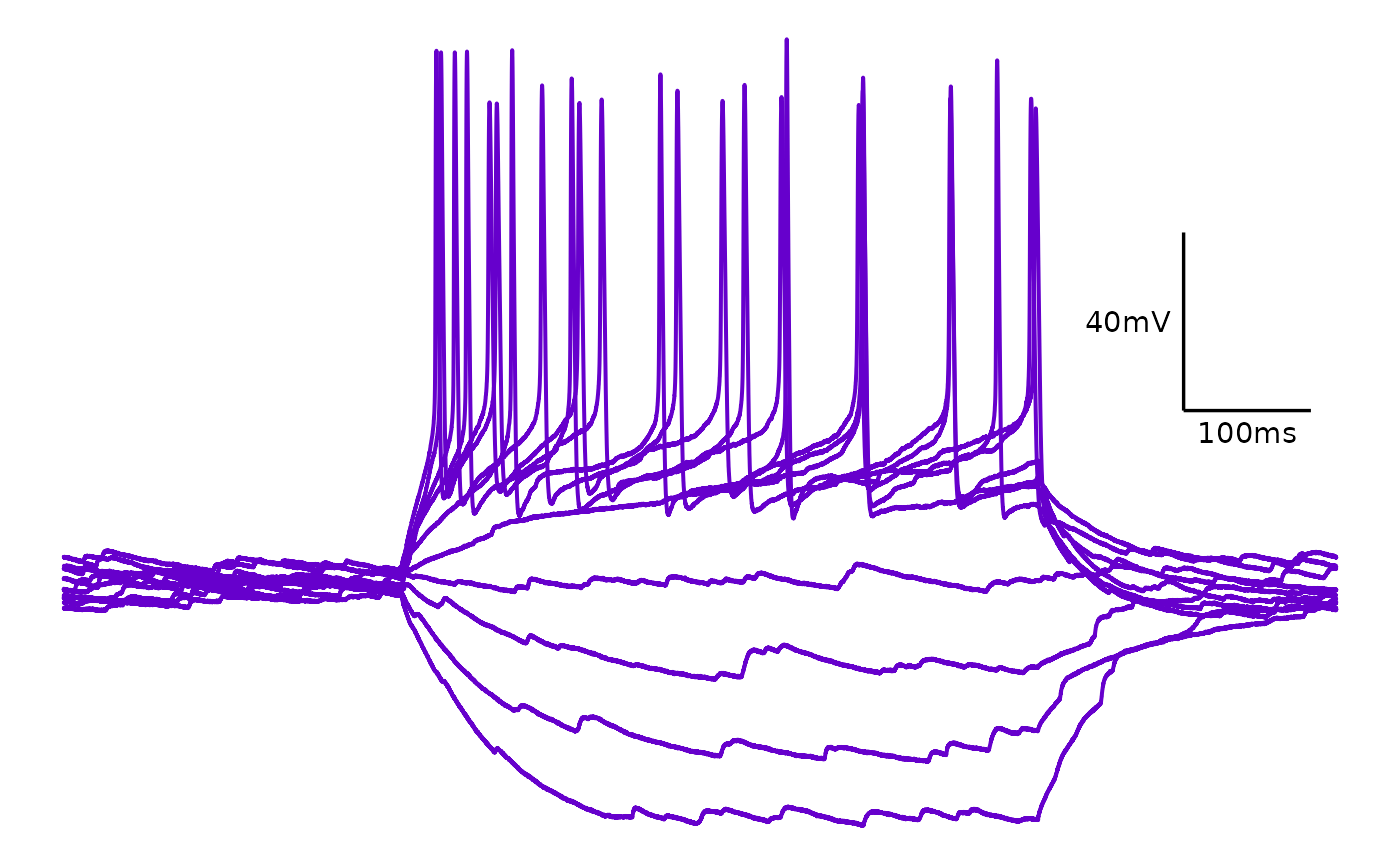
Single colour
plot_AP_trace(
  data = sample_ap_abf_baseline,
  sweeps = as.character(unique(sample_ap_abf_baseline$episode)),
  trace_colour = "#6600cc",
  colour_scale_option = "single_colour",
  plot_category = 2,
  plot_treatment = "Control"
)
FAQ
What do I do if there are no action potentials following treatment?
Do not discard this cell; this is important and meaningful data! Fill
in only the letter and state, and leave all other columns blank. R will
fill this with NA values, since there are no action potential properties
to measure. However, for your AP count data, please just indicate
0 for all current injections.
What do I do if there are action potentials outside of the time when a current injection was applied?
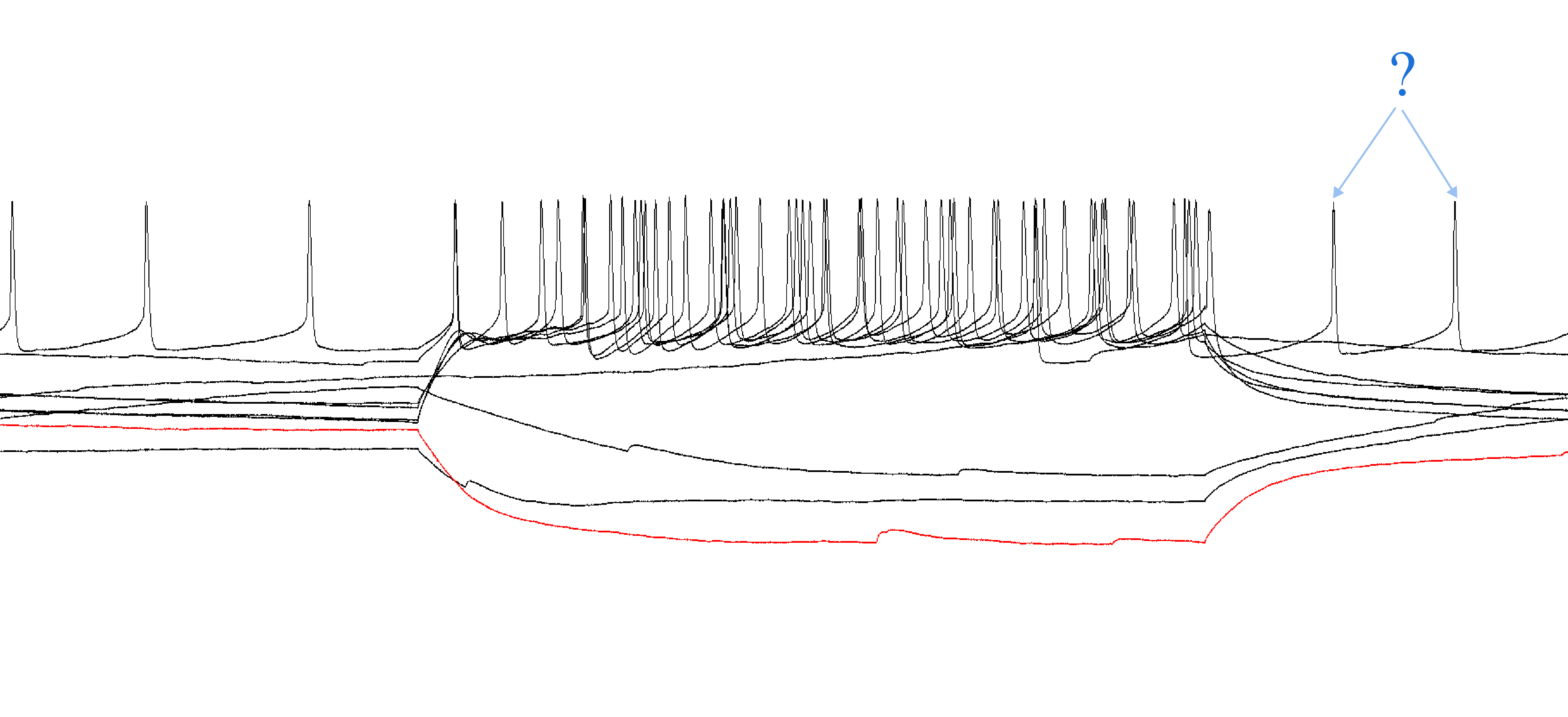
This can happen with very excitable cells. Only count the action potentials that occurred within the injection period.
Should I count an action potential that looks very wavy?

Only include the action potential if it clearly crosses the threshold, comes to a sharp peak, and has an after-hyperpolarization period.
References
Farries, M. A., Kita, H., & Wilson, C. J. (2010). Dynamic Spike Threshold and Zero Membrane Slope Conductance Shape the Response of Subthalamic Neurons to Cortical Input. Journal of Neuroscience, 30(39), 13180–13191. https://doi.org/10.1523/JNEUROSCI.1909-10.2010